AMP: mixed precision

⚠ INFORMATION
This page was translated by an AI (LLM) with a cursory human check and is awaiting full review.

Operating principle

The term precision here refers to the way real variables are stored in memory. Most of the time, real numbers are stored in 32 bits. They are called 32-bit floating-point reals, or float32, and we talk about single precision. Real numbers can also be stored in 64 or 16 bits, depending on the number of significant digits desired. We talk about float64 or double precision, and float16 or half precision, respectively. The TensorFlow and PyTorch frameworks use single precision by default, but it is possible to exploit half precision to optimise the learning step.

We talk about mixed precision when we combine several precisions in the same model during the forward and backward propagation steps. In other words, we reduce the precision of certain variables of the model during certain steps of the training.

It has been shown empirically that, even by reducing the precision of certain variables, we obtain a model learning equivalent in performance (loss, accuracy) as long as the "sensitive" variables retain the default float32 precision, and this for all current "major types" of models. In the TensorFlow and PyTorch frameworks, the "sensitive" nature of the variables is determined automatically thanks to the Automatic Mixed Precision or AMP feature. Mixed precision is a technique for optimising learning. At the end of this process, the trained model is converted back to float32, its initial precision.

Loss Scaling

It is important to understand the influence of converting certain model variables to float16 and not to forget to implement the Loss Scaling technique when using mixed precision.

Histogram of the most common values within the gradients of a neural network 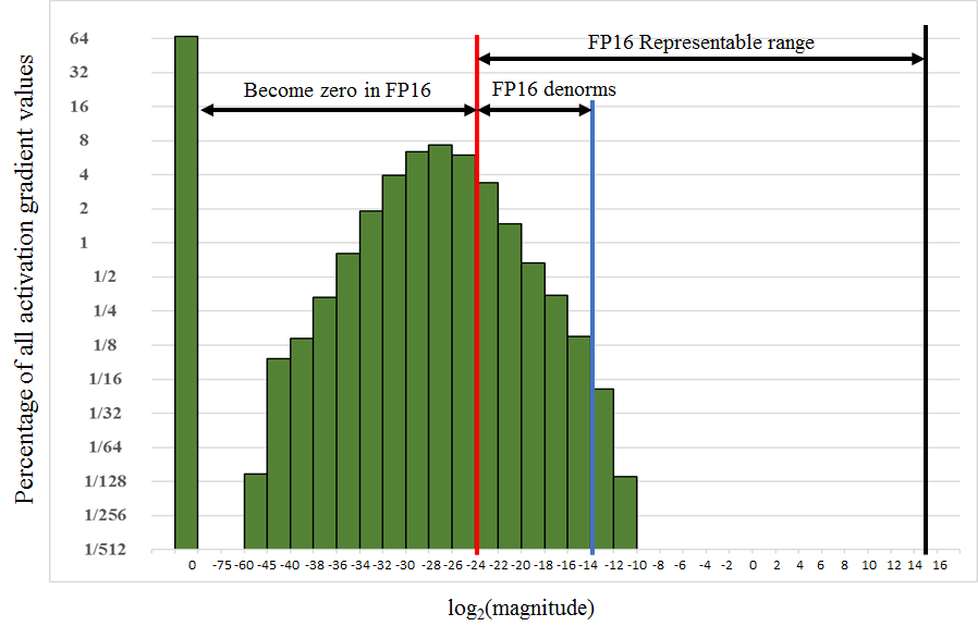Source: Mixed Precision Training

Indeed, the range of values representable in float16 precision extends over the interval [2-24,215]. However, as shown in the figure above, in some models, the gradient values are well below the range of values representable in float16 precision at the time of weight update. They are thus outside the representable range in float16 precision and are reduced to a null value. If nothing is done, the calculations risk being falsified while the range of values representable in float16 will remain largely unexploited.

To avoid this problem, a technique called Loss Scaling is used. During the learning iterations, the training Loss is multiplied by a factor S to shift the variables towards higher values, representable in float16. They will then need to be corrected before the model weight update, by dividing the weight gradients by the same factor S. This will restore the true gradient values.

To simplify this process, there are solutions in the TensorFlow and PyTorch frameworks to implement Loss scaling.

Benefits and constraints of mixed precision

Here are some advantages of exploiting mixed precision:

• Concerning memory:

  • The model takes up less space in memory since the size of certain variables is halved.
    warning

    The memory occupied is generally lower but not in all cases. Some variables are saved in both float16 and float32 and this duplication of data is not necessarily compensated by the reduction to float16 of the other variables.

  • As variables are faster to transfer in memory, the bandwidth is less stressed.

• Concerning calculations:

  • The training time is reduced.
  • On NVIDIA V100 GPUs, AMP allows the use of Tensor Cores and drastically reduces the calculation time by a factor of 2 or 3.

Among the classic examples of use, mixed precision allows to:

• reduce the memory size of a model (which would exceed the GPU memory size)
• reduce the training time of a model (such as large convolutional networks)
• double the batch size
• increase the number of epochs

There are few constraints to using AMP. A very slight decrease in the precision of the trained model can be noted (which is fully compensated by the gain in memory and calculation time) as well as the addition of a few lines of code.

AMP is a good practice to implement on Jean Zay!

Efficiency of AMP on Jean Zay

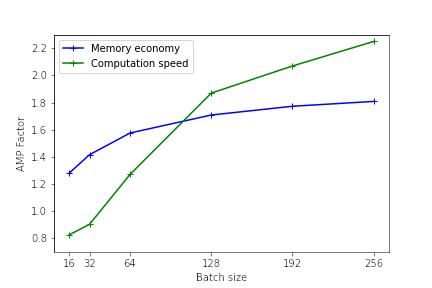
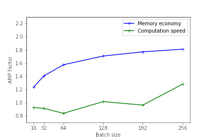
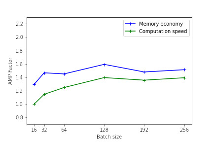
The following figures illustrate the memory and calculation time gains provided by the use of mixed precision as a function of the batch size. These results were measured on Jean Zay for the training of a Resnet50 model on CIFAR and executed in mono-GPU. (See the result of the 1st benchmark with Resnet101).

Pytorch mono-GPU V100

Pytorch mono-GPU A100

Tensorflow mono-GPU V100

Tensorflow mono-GPU A100

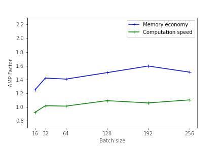
The heavier the model (in terms of memory and operations), the more effective the use of mixed precision will be. However, even for lighter models, there is an observable performance gain.

For the smallest models, the use of AMP is not beneficial. Indeed, the time taken to convert the variables can be greater than the gain achieved with the use of Tensor Cores.

Performance is better when the model dimensions (batch size, image size, embedded layers, dense layers) are multiples of 8, due to the hardware specificities of Tensor Cores as documented on the NVIDIA website.

note

These tests give an idea of the efficiency of AMP. The results may be different with other types and sizes of models. Implementing AMP remains the only way to know the real gain on your specific model.

Implementation with PyTorch

Since version 1.6, PyTorch includes functions for AMP (refer to the examples on the PyTorch page).

To implement mixed precision and Loss Scaling, a few lines need to be added:

from torch.cuda.amp import autocast, GradScaler

scaler = GradScaler()

for epoch in epochs:
    for input, target in data:
        optimizer.zero_grad()

        with autocast(device_type='cuda'):
            output = model(input)
            loss = loss_fn(output, target)

        scaler.scale(loss).backward()
        scaler.step(optimizer)
        scaler.update()

warning

Before version 1.11, in the case of distributed code with DataParallel, the use of autocast must be specified before the forwarding step in the model definition (see the fix on the PyTorch page). The use of a process per GPU with DistributedDataParallel is preferred over this solution.

note

NVIDIA Apex also offers AMP but this solution is now obsolete and discouraged.

Implementation with TensorFlow

Since version 2.4, TensorFlow includes a library dedicated to mixed precision:

from tensorflow.keras import mixed_precision

This library allows you to instantiate mixed precision in the backend of TensorFlow. The instruction is as follows:

mixed_precision.set_global_policy('mixed_float16')

warning

If you use a distribution strategy tf.distribute.MultiWorkerMirroredStrategy, the instruction mixed_precision.set_global_policy('mixed_float16') must be positioned inside the context with strategy.scope().

This tells TensorFlow to decide, at the creation of each variable, which precision to use according to the policy implemented in the library. The implementation of Loss Scaling is automatic when using keras. If you use a custom training loop with a GradientTape, you must explicitly apply the Loss Scaling after creating the optimiser and the steps of the Scaled Loss (refer to the page of the TensorFlow guide).