Data Parallelism with Horovod
Horovod is a software framework that enables data parallelism for TensorFlow, Keras, PyTorch, and Apache MXNet. Its goal is to improve code performance and make it easy to implement.
In the AI community examples, Horovod is often used with TensorFlow to simplify the implementation of data parallelism.
Horovod relies on the MPI and NCCL communication libraries to exchange data between compute processes.
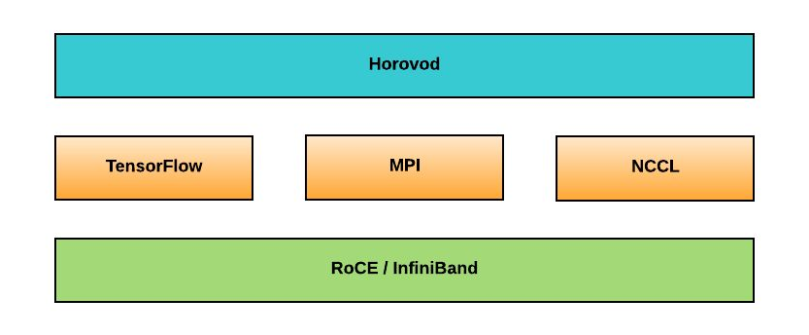 Horovod stack, also compatible with the PyTorch library
and the OmniPath interconnection network. Source.
Here, we document Horovod solutions on Jean Zay for TensorFlow and PyTorch. This is a multi-process parallelism that works equally well in single-node and multi-node configurations.
A practical example is provided as a Notebook below to give you access to a functional implementation of the explanations provided in this documentation.
Multi-Process Configuration with Slurm
One of the advantages of Horovod is that no manual configuration is required for the description of the distributed environment. Horovod directly retrieves information about the GPUs, available machines, and communication protocols from the machine environment. In particular, the Horovod solution ensures the portability of your code.
In Slurm, when you launch a script with the srun command, the script is automatically distributed across all predefined tasks. For example, if we reserve 4 nodes with 3 GPUs per node, we get:
- 4 nodes, indexed from 0 to 3
- 3 GPUs/node, indexed from 0 to 2 on each node
- 4 x 3 = 12 processes in total, allowing 12 tasks to be executed with ranks from 0 to 11
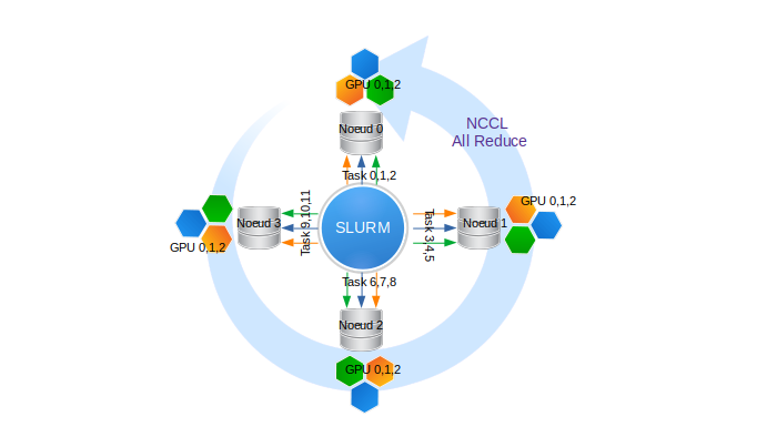
Illustration of a Slurm reservation with 4 nodes and 3 GPUs per node, i.e. 12 processes.
Inter-node collective communications are managed by the NCCL library.
To execute distributed code with Horovod under the Slurm environment, you must reserve one task per GPU involved in data parallelism.
Here are two example Slurm scripts for Jean Zay:
- for a reservation of N quad-GPU V100 nodes via the default GPU partition:
#!/bin/bash
#SBATCH --job-name=torch-multi-gpu
#SBATCH --nodes=N              # total number of nodes (N to be defined)
#SBATCH --ntasks-per-node=4    # number of tasks per node (here 4 tasks, i.e., 1 task per GPU)
#SBATCH --gres=gpu:4           # number of GPUs reserved per node (here 4, i.e., all GPUs)
#SBATCH --cpus-per-task=10     # number of cores per task (thus 4x10 = 40 cores, i.e., all cores)
#SBATCH --hint=nomultithread
#SBATCH --time=20:00:00
#SBATCH --output=torch-multi-gpu%j.out
##SBATCH --account=abc@v100

module load pytorch-gpu/py3/2.5.0

srun python myscript.py
- for a reservation of N octo-GPU A100 nodes:
#!/bin/bash
#SBATCH --job-name=torch-multi-gpu
#SBATCH --nodes=N            # total number of nodes (N to be defined)
#SBATCH --ntasks-per-node=8  # number of tasks per node (here 8 tasks, i.e., 1 task per GPU)
#SBATCH --gres=gpu:8         # number of GPUs reserved per node (here 8, i.e., all GPUs)
#SBATCH --cpus-per-task=8    # number of cores per task (thus 8x8 = 64 cores, i.e., all cores)
#SBATCH --hint=nomultithread
#SBATCH --time=20:00:00
#SBATCH --output=torch-multi-gpu%j.out
#SBATCH -C a100
##SBATCH --account=abc@a100

module load arch/a100
module load pytorch-gpu/py3/2.5.0

srun python myscript.py
In both examples, the nodes are reserved exclusively. In particular, this gives us access to all the memory on each node.
Implementing the Horovod Solution
Horovod can be used in the following software configurations:
- TensorFlow - See the Horovod TensorFlow documentation
- TensorFlow and Keras - See the Horovod with Keras documentation
- PyTorch - See the Horovod PyTorch documentation
We refer you to the Horovod documentation for implementation details related to each software configuration.
In all cases, the code differs slightly, but the development steps remain identical. You must:
- Import and initialise Horovod.
- Assign each GPU to a distinct process.
- Increase the learning rate proportionally to the number of GPUs to compensate for the increase in batch size.
- Distribute the optimiser.
- Ensure that the variables are correctly replicated across all GPUs at the start of training (and after model initialisation).
- Save checkpoints only from the rank 0 process.
For example, the Horovod solution implemented in a TensorFlow 2 + Keras code is illustrated in the following script:
import tensorflow as tf
import horovod.tensorflow.keras as hvd

# Initialise Horovod
hvd.init()

# Pin GPU to be used to process local rank (one GPU per process)
gpus = tf.config.experimental.list_physical_devices('GPU')
for gpu in gpus:
    tf.config.experimental.set_memory_growth(gpu, True)
if gpus:
    tf.config.experimental.set_visible_devices(gpus[hvd.local_rank()], 'GPU')

# Build model and dataset
dataset = ...
model = ...
opt = tf.optimizers.Adam(0.001 * hvd.size())

# Horovod: add Horovod DistributedOptimizer.
opt = hvd.DistributedOptimizer(opt)

# Horovod: Specify `experimental_run_tf_function=False` to ensure TensorFlow
# uses hvd.DistributedOptimizer() to compute gradients.
mnist_model.compile(loss=tf.losses.SparseCategoricalCrossentropy(),
                    optimizer=opt,
                    metrics=['accuracy'],
                    experimental_run_tf_function=False)

callbacks = [
    # Horovod: broadcast initial variable states from rank 0 to all other processes.
    # This is necessary to ensure consistent initialisation of all workers when
    # training is started with random weights or restored from a checkpoint.
    hvd.callbacks.BroadcastGlobalVariablesCallback(0),
]

# Horovod: save checkpoints only on worker 0 to prevent other workers from corrupting them.
if hvd.rank() == 0:
    callbacks.append(keras.callbacks.ModelCheckpoint('./checkpoint-{epoch}.h5'))

model.fit(dataset,
          steps_per_epoch=500 // hvd.size(),
          callbacks=callbacks,
          epochs=24,
          verbose=1 if hvd.rank() == 0 else 0)
Distributed Validation
The validation step, executed after each epoch or after a fixed number of training iterations, can be distributed across all GPUs involved in model training. When data parallelism is used and the validation dataset is large, this GPU-distributed validation solution appears to be the most efficient and fastest.
The challenge here is to compute the metrics (loss, accuracy, etc.) per batch and per GPU, then to weight and average them across the entire validation dataset.
To do this, you must:
- Load the validation data in the same way as the training data, but without random transformations such as data augmentation or shuffling (see the documentation on data loading for distributed training in TensorFlow):
# validation dataset loading (imagenet for example)val_dataset = tf.data.TFRecordDataset(glob.glob(os.environ['DSDIR']+'/imagenet/validation*'))# define distributed sharding for validationval_dataset = val_dataset.shard(hvd.size(), hvd.rank())# define dataloader for validationval_dataset = val_dataset.map(tf_parse_eval,num_parallel_calls=idr_tf.cpus_per_task).batch(batch_size).prefetch(buffer_size=5)
- Switch from 'training' to 'validation' mode to disable certain training-specific features that are costly and unnecessary here:
model(images, training=False)when evaluating the model, to switch the model to 'validation' mode and disable the management of dropout, batchnorm, etc.- Remove
tf.GradientTape()to skip gradient computation.
- Evaluate the model and compute the metric per batch in the usual way (here, we use the example of loss computation; the same applies to other metrics):
logits_ = model(images, training=False)followed byloss_value = loss(labels, logits_).
- Weight and accumulate the metric per GPU:
val_loss.update_state(loss_value, sample_weight=images.shape[0])whereimages.shape[0]is the batch size. Since batches may not all have the same size (the last batch is sometimes smaller), it is preferable to use the valueimages.shape[0]here.
- Compute the weighted averages of the metric across all GPUs:
hvd.allreduce(val_loss.result())to average the metric values computed per GPU and communicate the result to all GPUs. This operation involves inter-GPU communications. Horovod uses the average as the defaultallReduceoperation.
Example after loading the validation data:
loss = tf.losses.SparseCategoricalCrossentropy() # define loss function

val_loss = tf.keras.metrics.Mean()               # define Keras metrics

@tf.function                                     # define validation step function
def eval_step(images, labels):
    logits_ = model(images, training=False)      # evaluate model - switch into validation mode
    loss_value = loss(labels, logits_)           # compute loss
    val_loss.update_state(loss_value, sample_weight=images.shape[0]) # cumulative weighted mean per GPU

val_loss.reset_states()                          # initialise val_loss value

for val_images, val_labels in val_loader:
    eval_step(val_images, val_labels)            # call eval_step function

val_loss_dist = hvd.allreduce(val_loss.result()) # average weighted means and broadcast value to each GPU
SyncBatchNorm for Data Parallelism
BatchNorm layers allow for faster model training by having it converge quicker towards a better optimum. See the reference article on layer normalisation
BatchNormalization layers apply a transform which maintains previous layer outputs mean at 0 and standard deviation at 1. In other words, they compute normalisation factors in order to normalise the output of every layer (or only some layers) of the model. Those factors are learned during training: at every step (the pass of a single batch), the BatchNormalization layer also learns the mean and standard deviation of the batch (for each dimension). The combination of these factors allow the mean and standard deviation to stay close to 0 and 1, respectively.
Batch Normalization behaves differently during training, validation, and inference. Therefore, it is important to indicate to the model its current state (training or validation).
During training, the layer normalises its outputs using the mean and standard deviation of the input batch. More precisely, the layer returns (batch - mean(batch)) / (var(batch) + epsilon) * gamma + beta, with:
epsilon, a small constant to avoid division by zero,gamma, a learned (trained) parameter updated via gradient calculation during backpropagation, initialised to 1,beta, a learned (trained) parameter updated via gradient calculation during backpropagation, initialised to 0.
During inference or validation, the layer normalises its outputs using the trained gamma and beta, along with the moving_mean and moving_var factors: (batch - moving_mean) / (moving_var + epsilon) * gamma + beta.
moving_mean and moving_var are non-trainable factors, but they are updated at each batch iteration during training according to the following method:
moving_mean = moving_mean * momentum + mean(batch) * (1 - momentum)moving_var = moving_var * momentum + var(batch) * (1 - momentum)
SyncBatchNorm Layers
In data parallelism, a replica of the model is loaded onto each device (GPU). These replicas are intended to be completely equivalent across all devices. However, with Batch Normalization, and because each parallelised device processes different mini-batches, the normalisation statistics are likely to diverge, particularly the moving_mean and moving_var variables.
If the mini-batch sizes per GPU are sufficiently large, this divergence may be considered acceptable. However, it is recommended and sometimes necessary to replace BatchNorm layers with SyncBatchNorm layers.
SyncBatchNorm layers enable synchronisation across devices (during data parallelism) for the computation of normalisation statistics.
SyncBatchNorm with Horovod
As of now, Horovod does not officially document the use of SyncBN layers. However, they are available for TensorFlow and PyTorch.
Practical Example
An example can be found in $DSDIR/examples_IA/Horovod_parallel/Example_DataParallelism_Horovod_Tensorflow-eng.ipynb on Jean Zay. It uses the MNIST dataset and a simple dense network.
The example is a Notebook that allows you to create an execution script. It should be copied to your personal space (ideally to your $WORK):
cp $DSDIR/examples_IA/Horovod_parallel/Example_DataParallelism_Horovod_Tensorflow-eng.ipynb $WORK
You can then run the Notebook from a Jean Zay login node by selecting a PyTorch or TensorFlow kernel (see our JupyterHub access documentation for more information on using Notebooks on Jean Zay).