Profiling of PyTorch Applications
This page was translated by an AI (LLM) with a cursory human check and is awaiting full review.
We present here how to instrument your PyTorch code with the profiler integrated into the library and different ways to visualise the generated traces.
Instrumenting PyTorch code for profiling
In PyTorch code, you must first import and define the desired type of monitoring when defining the profiler:
from torch.profiler import profile, tensorboard_trace_handler, ProfilerActivity, schedule

prof = profile(activities=[ProfilerActivity.CPU, ProfilerActivity.CUDA], # 1
               schedule=schedule(wait=1, warmup=1, active=12, repeat=1), # 2
               on_trace_ready=tensorboard_trace_handler(logname),        # 3
               profile_memory=True,                                      # 4
               record_shapes=False,                                      # 5
               with_stack=False,                                         # 6
               with_flops=False)                                         # 7
where:
- activities=[ProfilerActivity.CPU, ProfilerActivity.CUDA]: allows monitoring of both CPU and GPU activity;
- schedule=[...]: allows defining a profiling cycle. The first step is generally ignored as it is not representative (
wait=1), an additional time is defined for the initialisation of CUDA monitoring tools (warmup=1), only a few steps are monitored (here 12 steps withactive=12) and the number of times the cycle should be repeated is defined (once here withrepeat=1); - on_trace_ready=tensorboard_trace_handler(logname): allows storing logs in a json format compatible with the TensorBoard plugin;
- profile_memory=True: allows retrieving memory traces;
- record_shapes=True: allows retrieving the format of tensors as inputs to functions;
- with_stack=True: allows keeping the call stack;
- with_flops: allows retrieving an estimate of the FLOPs performance of tensor operations.
- Profiling is an expensive operation, usually performed on only a few steps.
- Keeping the call stack with
with_stack=Truesignificantly increases the size of the logs.
You must then invoke the profiler at the beginning of the training loop and indicate the end of the step by calling prof.step():
with prof:
    for epoch in range(args.epochs):
        for i, (samples, labels) in enumerate(train_loader):
            ...
            prof.step() # Need to call this at the end of each step to notify profiler of steps' boundary.
It is possible to customise profiling by integrating record_function decorators around areas of interest. For example:
from torch.profiler import profile, record_function, ProfilerActivity
...
with profile(activities=[ProfilerActivity.CPU, ProfilerActivity.CUDA], record_shapes=True) as prof:
    with record_function("Training loop"):
        train()
...
def train():
    for epoch in range(1, num_epochs+1):
        for i_step in range(1, total_step+1):
            # Obtain the batch.
            with record_function("Loading input batch"):
                images, captions = next(iter(data_loader))
            ...
            with record_function("Training step"):
              ...
                loss = criterion(outputs.view(-1, vocab_size), captions.view(-1))
              ...
Visualisation of traces
Basic visualisation
You can request the display of a summary table of the profiling traces at the end of the script by adding the following line:
print(prof.key_averages().table(sort_by="cpu_time", row_limit=10))
with:
sort_byallowing sorting of functions by category (for example:<device>_time,self_<device>_time_total,<device>_time_total,self_<device>_memory_usage,<device>_memory_usage);row_limit=Nallowing limiting the display to the first N functions.
You get a list of automatically tagged functions or tagged by us (via decorators) sorted in the desired order. For example:
-------------------------------------------------------  ------------  ------------  ------------  ------------  ------------  ------------  ------------  ------------  ------------  ------------  ------------  ------------  ------------  ------------
                                                   Name    Self CPU %      Self CPU   CPU total %     CPU total  CPU time avg     Self CUDA   Self CUDA %    CUDA total  CUDA time avg       CPU Mem  Self CPU Mem      CUDA Mem  Self CUDA Mem    # of Calls
-------------------------------------------------------  ------------  ------------  ------------  ------------  ------------  ------------  ------------  ------------  ------------  ------------  ------------  ------------  ------------  ------------
                                          ProfilerStep*        30.66%     434.580ms        75.83%        1.075s      89.576ms       0.000us         0.00%     398.617ms      33.218ms           0 B          -8 B      99.24 MB     -39.20 GB            12
                        DistributedDataParallel.forward         4.68%      66.296ms        21.15%     299.826ms      24.986ms       0.000us         0.00%     328.890ms      27.408ms           0 B           0 B      39.87 GB      -2.71 GB            12
                                             aten::item         0.01%     123.548us        16.79%     238.018ms       9.917ms       0.000us         0.00%      37.216us       1.551us           0 B           0 B           0 B           0 B            24
                              aten::_local_scalar_dense         0.04%     512.303us        16.78%     237.895ms       9.912ms      37.216us         0.00%      37.216us       1.551us           0 B           0 B           0 B           0 B            24
                                  cudaStreamSynchronize        16.69%     236.618ms        16.70%     236.786ms       9.866ms       0.000us         0.00%       0.000us       0.000us           0 B           0 B           0 B           0 B            24
                       Runtime Triggered Module Loading         2.08%      29.521ms         2.08%      29.521ms       7.380ms       1.415ms         0.15%       1.415ms     353.807us           0 B           0 B           0 B           0 B             4
                                Optimizer.step#SGD.step         0.99%      14.036ms         4.78%      67.830ms       5.653ms       0.000us         0.00%      15.416ms       1.285ms           0 B           0 B      99.61 MB           0 B            12
                                    aten::_foreach_mul_         0.47%       6.731ms         1.32%      18.778ms       1.707ms       3.337ms         0.36%       4.255ms     386.783us           0 B           0 B           0 B           0 B            11
                                    aten::_foreach_add_         0.70%       9.947ms         2.06%      29.251ms       1.272ms       9.423ms         1.01%      10.628ms     462.097us           0 B           0 B           0 B           0 B            23
                                Activity Buffer Request         0.08%       1.106ms         0.08%       1.106ms       1.106ms       1.152us         0.00%       1.152us       1.152us           0 B           0 B           0 B           0 B             1
-------------------------------------------------------  ------------  ------------  ------------  ------------  ------------  ------------  ------------  ------------  ------------  ------------  ------------  ------------  ------------  ------------
Self CPU time total: 1.418s
Self CUDA time total: 935.789ms
TensorBoard plugin
The traces generated by the PyTorch profiler can be visualised with the TensorBoard plugin torch_tb_profiler.
The plugin torch_tb_profiler remains usable but is no longer maintained. Users are officially referred to the alternative use of the HTA library, but this does not offer the same functionalities.
Visualisation of the traces is possible on the IDRIS JupyterHub platform, by opening TensorBoard according to the procedure described on this page.
You can also open the traces on your local machine if you wish. You must first have installed the plugin: pip install torch_tb_profiler. TensorBoard then opens as usual: tensorboard --logdir <profiler log directory>.
In the PYTORCH_PROFILER tab, you will find different views:
- Overview
- Operator view
- Kernel view
- Trace view
- Memory view, if the
profile_memoryoption has been activated in the Python code - Distributed view, if the code is distributed over several GPUs
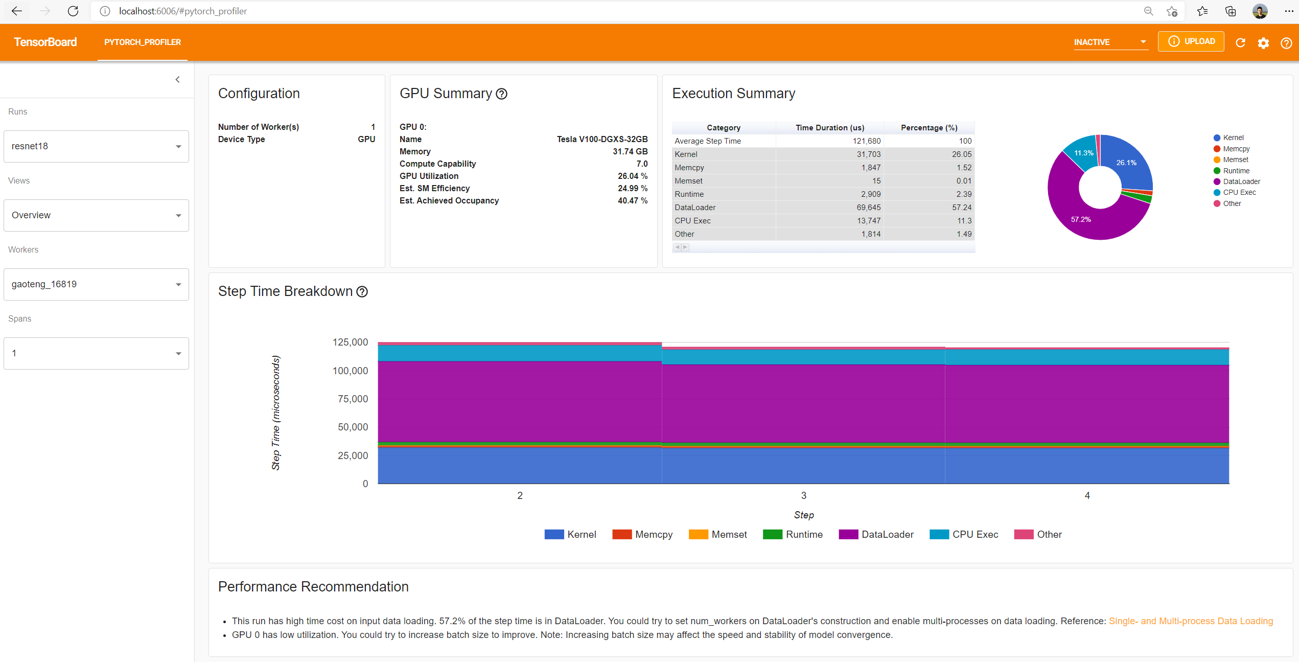
Onglet Overview
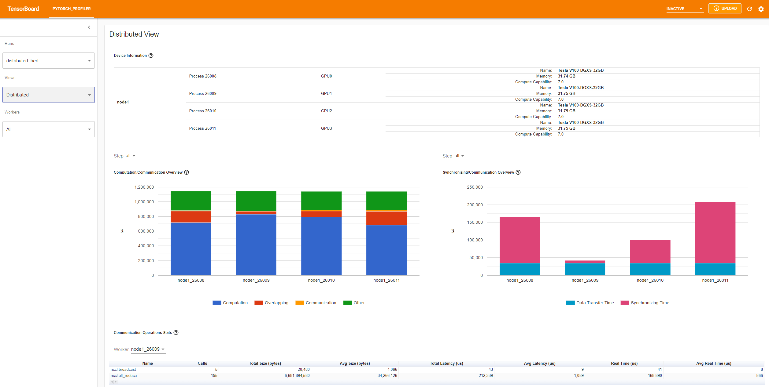
Onglet Distributed view
Since pytorch 1.10.0, information on the use of Tensor Cores is present on Overview, Operator view and Kernel View.
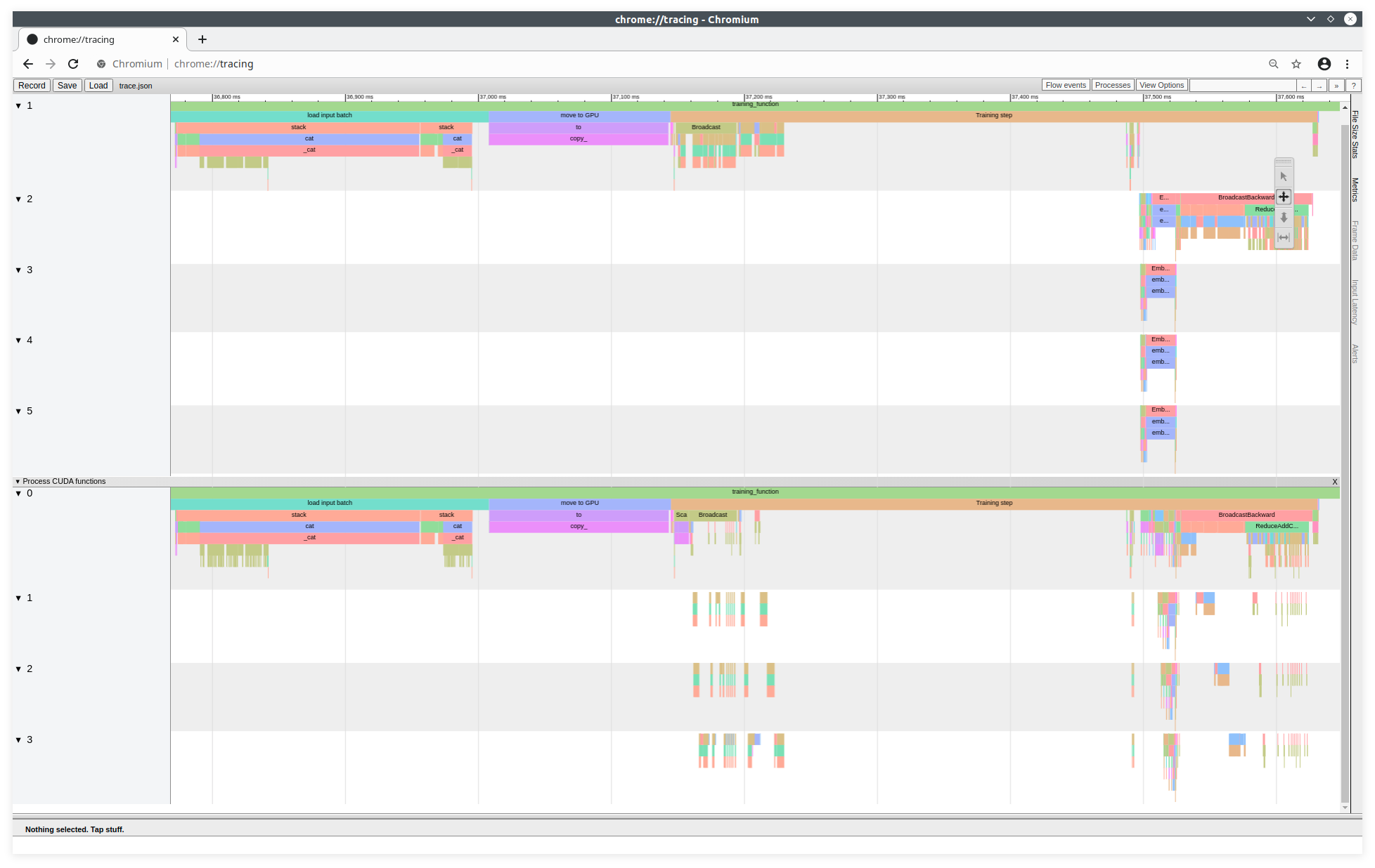
Chromium tracing
To display a Trace Viewer equivalent to that of TensorBoard, you can also generate a json trace file with the following line:
prof.export_chrome_trace("trace.json")
This trace file can be viewed on the Chromium project's trace tool. From a CHROME (or CHROMIUM) browser, you need to run the following command in the URL bar:
about:tracing
Example of a trace from the Chromium tool