Jean Zay: Multi-GPU and multi-node distribution for training a TensorFlow or PyTorch model

The training of a neural network model is faced with two major problems:

• The training time can be very long (several weeks).
• The model can be too large for the GPU memory (32 GB or 16 GB, depending on the partition used).

The solution to these two problems can be found in multi-GPU distribution. We distinguish between two techniques:

• Data parallelism which accelerates the model training by distributing each batch of data and therefore, each iteration upgrade of the model. In this case, the model is replicated on each utilised GPU to treat a data subset. It is adapted to trainings involving voluminous data or large-sized batches. This is the most documented distribution process and is the easiest one to implement.
• Model parallelism which is adapted to models which are too large to be replicated and manipulated with the chosen batch size in each GPU. However, it is more difficult to implement, particularly in multi-nodes. It can be optimised with pipeline techniques but it cannot accelerate the training as significantly as data parallelism.

These two techniques can be used simultaneously (hybrid parallelism) to solve both problems at the same time (training time and model size) by grouping the GPUs in function of the task to be effectuated.

Data parallelism consists of replicating the model on all the GPUs and dividing the data batch into mini-batches. Each GPU takes charge of a mini-batch, resulting in parallel learning on the entirety of the mini-batches.

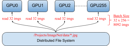
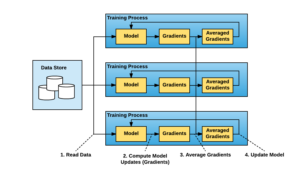
1. The training script is executed in distributed mode on several workers (i.e. several GPUs or several groups of GPUs). In this way, each GPU :
   1. Reads a part of the data (mini-batch).
   2. Trains the model from its mini-batch.
   3. Calculates the parameter updates of the local model (local gradients).
2. The global gradients are calculated from averaging the local gradients returned by all the GPUs. At this step, it is necessary to synchronise the different workers.
3. The model is updated on all the GPUs.
4. The algorithm is repeated beginning with step 1.a. until the end of the training.

• Implementation with PyTorch
• Implementation with Horovod
• Implementation with TensorFlow
• Implementation with Pytorch Lightning

Caution: This can be difficult to put in place because it requires, at minimum, the definition of a superclass for the model or the complete re-definition of the model sequentially. It would be preferable to use other optimisations to address the problems of memory occupation (Gradient Checkpointing, ZeRO of DeepSpeed, …). Only very big models (for example, for the most efficient transformers) will use model parallelism by absolute necessity.

Model parallelism consists of splitting a model onto more than one GPU in order to:

• Limit the volume of calculations to be effectuated by a single GPU during the training.
• To reduce the memory footprint of the model on each GPU (necessary for models which are too big to fit into the memory of a single GPU). In theory, the memory occupancy per GPU is thus divided by the number of GPUs.

The model is divided into groups of successive layers and each GPU takes charge of only one of these groups; this limits the number of parameters to process locally.

Unlike data parallelism, it is not necessary to synchronise the gradients: The GPUs collaborate sequentially to effectuate the training on each data input. The following figure illustrates model parallelism on 2 GPUs, thus dividing by 2 the size of the memory consumed in one GPU.

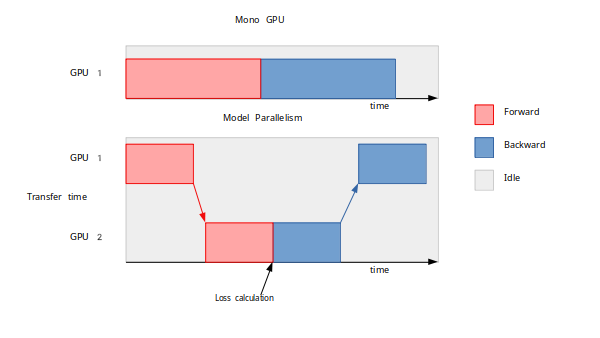
Note that model parallelism does not accelerate the learning because a GPU must wait for preceding layers of the model to be treated by another GPU before being able to execute its own layers. The learning is even a little longer because of the time of data transfer between GPUs.

Nevertheless, it is possible to decrease the time through process optimisation using a data pipeline technique: batch splitting. This consists of dividing the batch into micro-batches in order to limit the wait time and have the GPUs work quasi-simultaneously. However, there will still be a small wait time (the Bubble in the illustration).

The illustration below shows the quasi-simultaneity and the gain obtained by using the splitting technique where the data batch is divided into 4 micro-batches, for a training distributed on 4 GPUs.

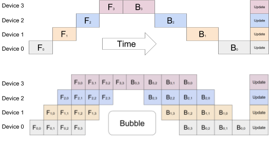
The optimal number of micro-batches depends on the model under consideration.

• Model parallelism with PyTorch
• Data and model parallelism with PyTorch

• Use DeepSpeed, the PyTorch optimisation library for big models
  • Optimal acceleration of learning and memory efficiency
  • ZeRO, ZeRO Offload and ZeRO Infinity
  • Activation checkpointing (equivalent to gradient checkpointing)
  • Optimisers
• Use PyTorch Lightning, the PyTorch simplification for high performance AI research
  • Simplification and good practices
  • Sharded training (equivalent to ZeRO)
  • Model parallelism
  • DeepSpeed plugin
  • Profiler
• Read theTensorFlow guide on optimising GPU performance.
• Read the NVIDIA guide on optimising GPU performance.

• TensorFlow Guide
• PyTorch Model Parallelism tutorial
• PyTorch Data Parallelism tutorial
• Understanding Scalability and Fine-Grain Parallelism of Synchronous Data Parallel Training
• Horovod: Fast and easy distributed deep learning in TensorFlow
• Demystifying Parallel and Distributed Deep Learning: An In-Depth Concurrency Analysis

* Introducing GPipe, an Open Source Library for Efficiently Training Large-scale Neural Network Models