

Table des matières
PyTorch: Multi-GPU model parallelism
The methodology presented on this page shows how to adapt, on Jean Zay, a model which is too large for use on a single GPU with PyTorch. This illustates the concepts presented on the main page: Jean Zay: Multi-GPU and multi-node distribution for training a TensorFlow or PyTorch model. We will only look at the optimized version of model parallelism (Pipeline Parallelism) as the naive version is not advised.
The PyTorch documentation is very complete on this subject: You only need to make some small modifications for the parallelism model to work with batch segmentation (Pipeline Parallelism) on Jean Zay. If you are just starting out with model parallelism, we advise you to first look at the PyTorch tutorial on this subject.
This document only presents the changes to be made in order to parallelize a model on Jean Zay and provides a benchmark to give an idea of the optimization of the method parameters. A complete demonstration (which has served as the benchmark) is found in a python code which is downloadable here or recoverable on Jean Zay in the DSDIR directory: $DSDIR/examples_IA/Torch_parallel/bench_PP_transformer.py.
To copy it into your $WORK space:
$ cp $DSDIR/examples_IA/Torch_parallel/demo_model_parallelism_pytorch.ipynb $WORK
There are other methods for implementing model parallelism which are explained in the following link: Single-Machine Model Parallel Best Practices. However, they seem to be less effective than the method presented on this page.
Configuration of the Slurm computing environment
Only one task must be instantiated for a model (or group of models) and an adequate number of GPUs which must all be on the same node. If we take an example of a model which we want to distribute on 4 GPUs, the following options are required:
#SBATCH --gres=gpu:4
#SBATCH --ntasks-per-node=1
The methodology presented, which only relies on the PyTorch library, is limited to mono-node multi-GPU parallelism (of 2 GPUs, 4 GPUs or 8 GPUs) and cannot be applied to a multi-node case. It is strongly recommended to associate this technique with data parallelism, as described on the page Parallelism of data and model with PyTorch, in order to effectively accelerate the trainings.
If your model requires model parallelism on more than one node, we recommend that you explore the solution documented on the page Distributed Pipeline Parallelism Using RPC.
Benchmark
A benchmark was created to compare Pipeline Parallelism (with different parameters) with the naive model parallelism. Tests were carried out on 2 and 4 GPUs; therefore with a model cut into two or four parts. The model used is a transformer which is trained on the IMDB Review dataset (the goal is to measure the training performances; using a transformer for an uncomplicated task is not advised). Different batch sizes were also tested, from 32 to 256, combined with different chunks, from 1 (naive parallelism) to 16. The results are the following (when a sample is missing, it is because there was an OOM):
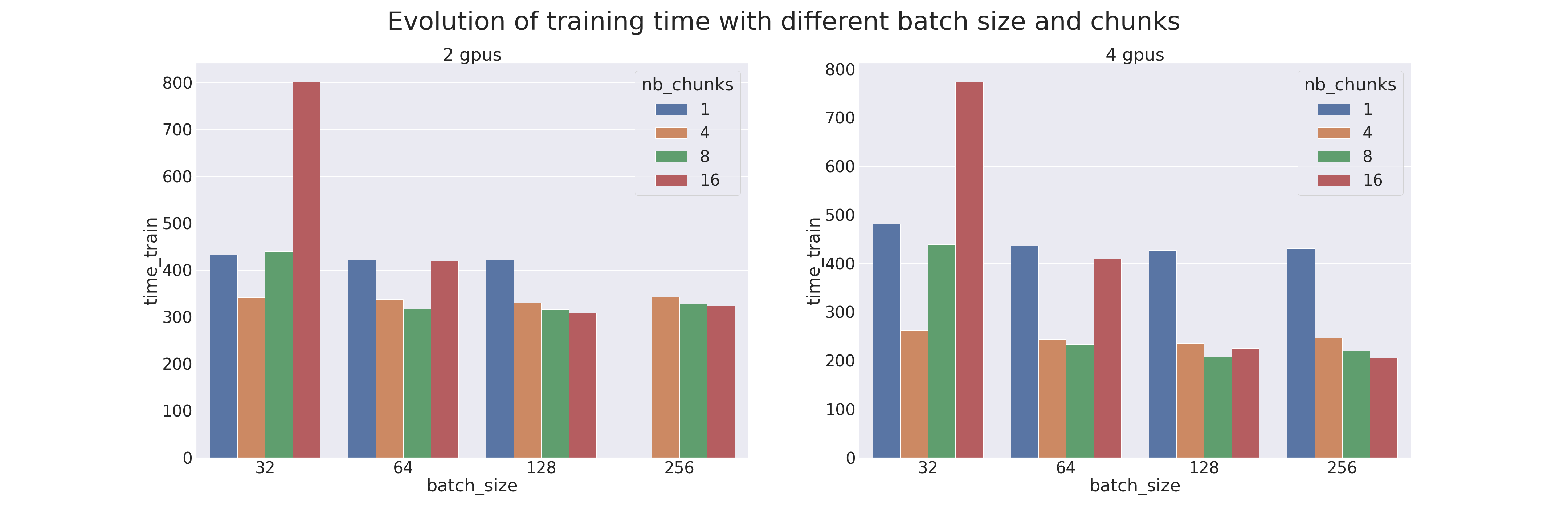
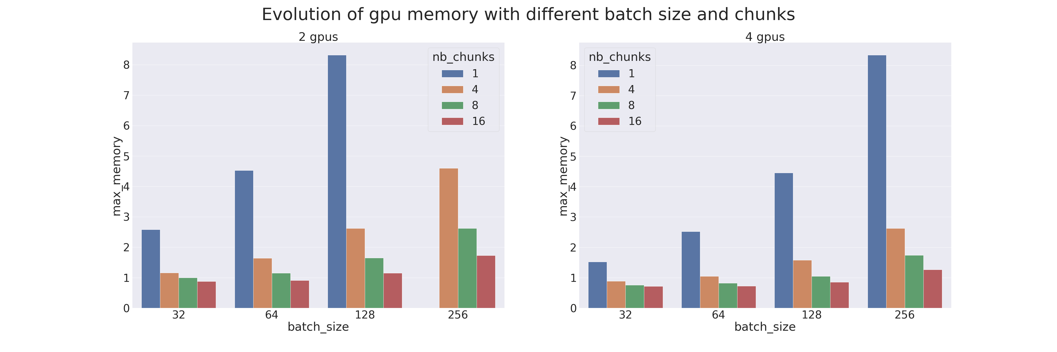
We see that Pipeline Parallelism is always more efficient (in execution time and in memory) than the Model Parallelism when the right chunk is found. Therefore, it is necessary to correctly accord the number of chunks with the batch size. Attention: the memory gain is due to the gradient checkpointing applied by default on the Pipe models.