Jean Zay: PyTorch profilers, native and with TensorBoard

PyTorch proposes different types of integrated profilers, depending on the version. This page describes the profiler built on TensorBoard and the preceding profiler called “native” which is visualized in another way.

Beginning with version 1.9.0, PyTorch integrates the PyTorch Profiler functionality as a TensorBoard plugin.

In the PyTorch code, you must:

• Import the profiler.

from torch.profiler import profile, tensorboard_trace_handler, ProfilerActivity, schedule

• Then invoke the profiler during the execution of the training loop with a prof.step() at the end of each iteration.

with profile(activities=[ProfilerActivity.CPU, ProfilerActivity.CUDA], # (1)
             schedule=schedule(wait=1, warmup=1, active=5, repeat=1),  # (2)
             on_trace_ready=tensorboard_trace_handler(logname),        # (3)
             profile_memory=True,                                      # (4)
             record_shapes=False,                                      # (5)
             with_stack=False,                                         # (6)
             with_flops=False)                                         # (7)
                    ) as prof:
    for epoch in range(args.epochs):
        for i, (samples, labels) in enumerate(train_loader):
 
            ...
 
            prof.step() # Need to call this at the end of each step to notify profiler of steps' boundary.

The above definition means:

• (1) We monitor the activity both on CPUs and GPUs.
• (2) We ignore the first step (wait=1) and we initialize the monitoring tools on one step (warmup=1). We activa)te the monitoring on 5 steps (active=5) and repeat the pattern only once (repeat=1).
• (3) We store the traces in a TensorBoard format (.json).
• (4) We profile the memory usage (significantly increases the traces size).
• (5) We don’t record the input shapes of the operators.
• (6) We don’t record call stacks (information about the active subroutines).
• (7) We don’t request the FLOPs estimate of the tensor operations.

• On the IDRIS JupyterHub, visualization of the traces is possible by opening TensorBoard according to the procedure described on the following page.

• Alternatively on your local machine, with the installation of the TensorBoard plugin, you can visualize the profiling traces. This is done as follows:

   pip install torch_tb_profiler 

After this, you only need to launch TensorBoard in the usual way with the command:

tensorboard --logdir <profiler log directory> 

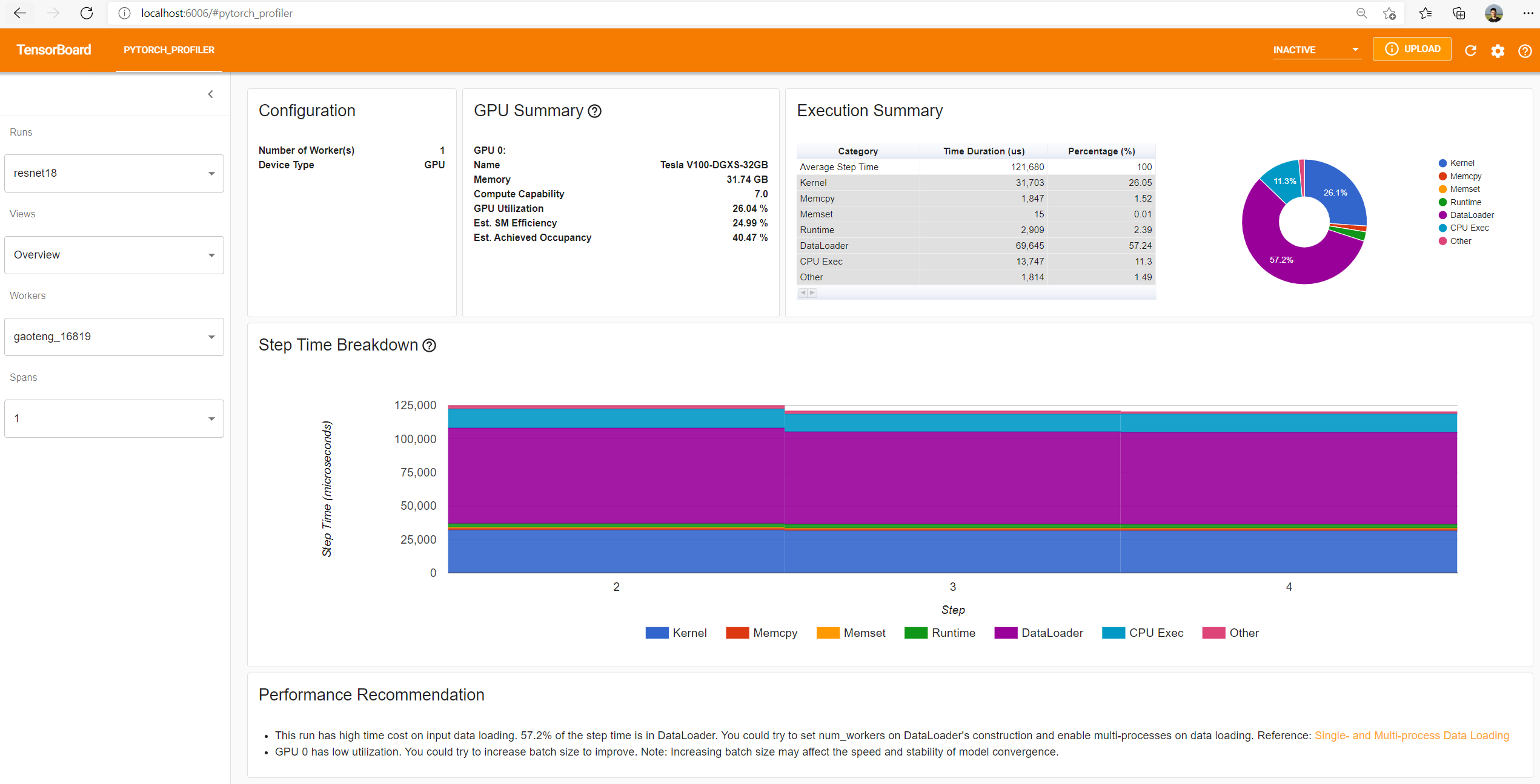
In the PYTORCH_PROFILER tab, you will find different views:

• Overview
• Operator view
• Kernel view
• Trace view
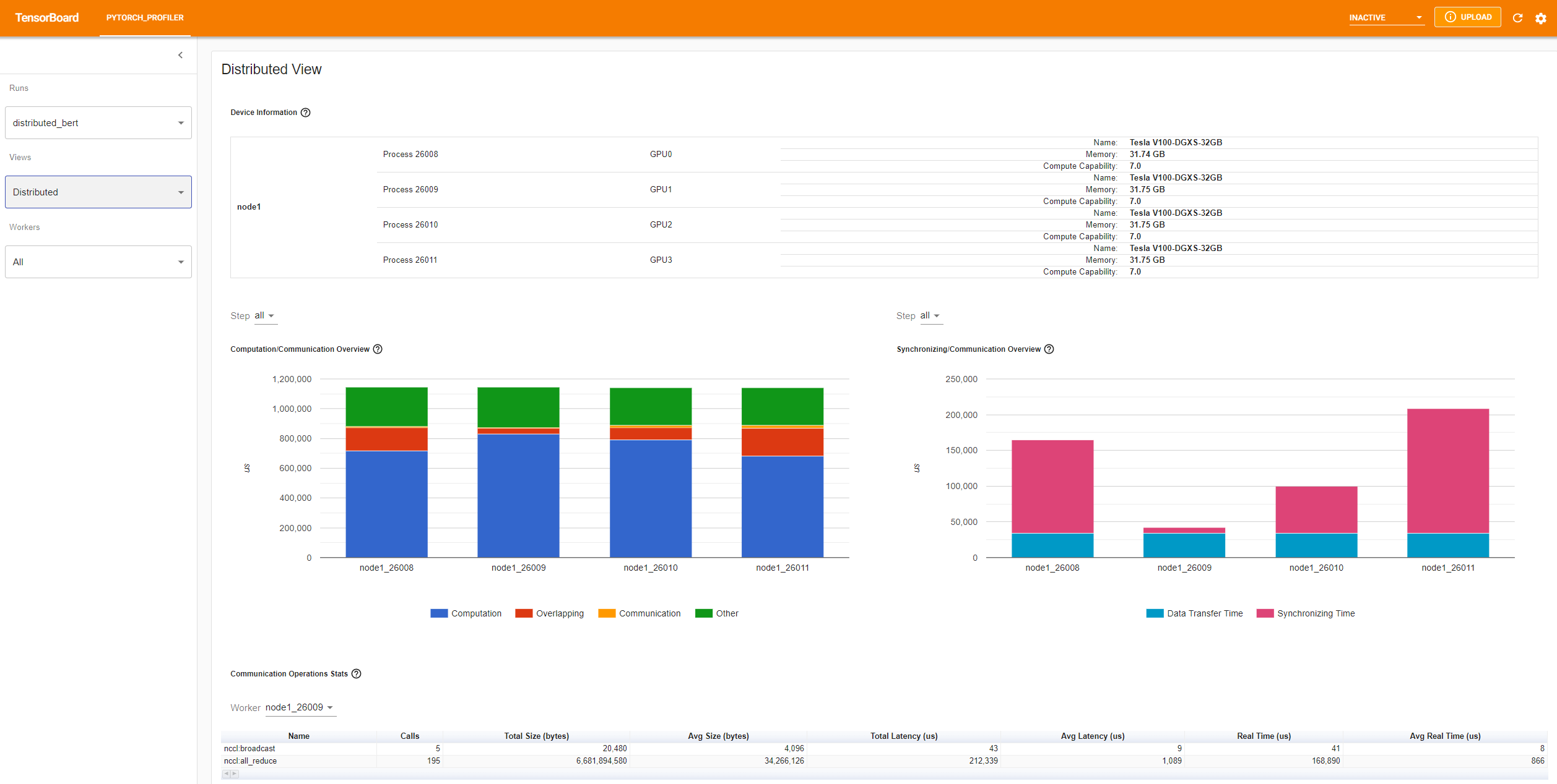
• Memory view, if the profile_memory=True option was instrumented in the python code.
• Distributed view, if the code is distributed on multiple GPUs.

For reasons of simplicity, or the need to use an earlier Pytorch version, you can also use the native PyTorch profiler.

In the PyTorch code, it is necessary to:

• Import the profiler.

from torch.profiler import profile, record_function, ProfilerActivity

• Then invoke the profiler during the execution of the training function.

with profile(activities=[ProfilerActivity.CPU, ProfilerActivity.CUDA], record_shapes=True) as prof:
    with record_function("training_function"):
        train()

Comments :

• ProfilerActivity.CUDA: Allows recovering the CUDA events (linked to the GPUs).
• With record_function(“$NAME”): Allows putting a decorator (a tag associated to a name) for a block of functions. Therefore, it is also useful to put decorators in the training function for the sets of sub-functions. For example:

def train():
    for epoch in range(1, num_epochs+1):
        for i_step in range(1, total_step+1):
            # Obtain the batch.
            with record_function("load input batch"):
                images, captions = next(iter(data_loader))
            ...
            with record_function("Training step"):
              ...
                loss = criterion(outputs.view(-1, vocab_size), captions.view(-1))
              ...

• Starting with PyTorch version 1.6.0, it is possible to profile the CPU and GPU memory footprint by adding the profile_memory=True parameter under profile.

To display the profiling results after the training function has executed, you must launch the following line:

print(prof.key_averages().table(sort_by="cpu_time", row_limit=10))

You will then obtain a table showing all the automatically tagged functions or those tagged yourself (via decorators), listing the total CPU times in descending order. For example:

|-----------------------------------   ---------------  ---------------  -------------  -------------- 
Name                                   Self CPU total   CPU total        CPU time avg  Number of Calls 
|-----------------------------------   ---------------  ---------------  -------------  -------------- 
training_function                     1.341s            62.089s          62.089s          1                
load input batch                      57.357s           58.988s          14.747s          4                
Training step                         1.177s            1.212s           303.103ms        4                
EmbeddingBackward                     51.355us          3.706s           231.632ms        16               
embedding_backward                    30.284us          3.706s           231.628ms        16               
embedding_dense_backward              3.706s            3.706s           231.627ms        16               
move to GPU                           5.967ms           546.398ms        136.599ms        4                
stack                                 760.467ms         760.467ms        95.058ms         8                
BroadcastBackward                     4.698ms           70.370ms         8.796ms          8                
ReduceAddCoalesced                    22.915ms          37.673ms         4.709ms          8                
|-----------------------------------  ---------------   ---------------  ---------------  ------------

The “Self CPU total” column shows the time spent in the function itself, but not in its sub-functions.

The “Number of Calls” column shows the number of GPUs used by a function.

In the table, we see that the time for loading the images (the load input batch step) is much larger than the neural network training (Training step). The optimization work should, therefore, target batch loading.

To display a Trace Viewer equivalent to that of TensorBoard, you can generate a “json” trace file with the following line:

prof.export_chrome_trace("trace.json")

This trace file is viewable on the Chromium project trace tool. From a CHROME (or CHROMIUM) browser, you need to launch the following command in the URL bar:

about:tracing    

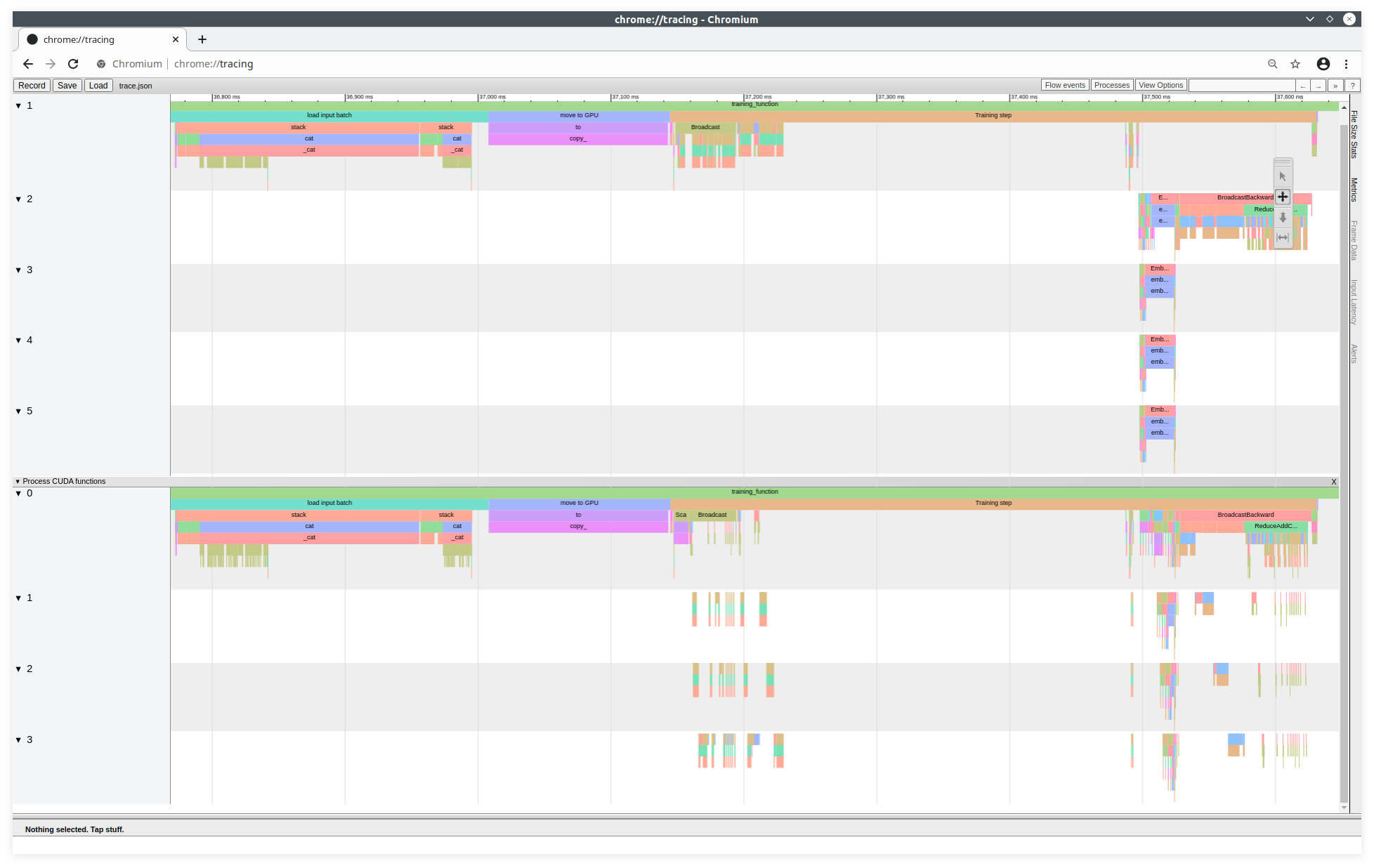
Here we distinctly see the CPU and GPU usage, as with TensorBoard. The CPU functions are shown on the top and the GPU functions are on the bottom. There are 5 CPU tasks and 4 GPU rasks. Each block of colour represents a function or a sub-function. We are at the end of a loading.

• Profiling a PyTorch code : https://pytorch.org/tutorials/recipes/recipes/profiler.html, https://pytorch.org/docs/stable/autograd.html, https://pytorch.org/tutorials/intermediate/tensorboard_profiler_tutorial.html

⇐ Return to the page on profiling applications