

Jean Zay: TensorFlow and PyTorch profiling tools
Profiling is an indispensable step in code optimization. Its goal is to target the execution steps which are the most costly in time or memory and to visualize the workload distribution among GPUs and CPUs.
Profiling an execution is a very time-consuming operation. Therefore, this is generally done on only a few iterations of your training steps. The creation of logs is done a posteriori, at the end of the job. It is not possible to visualize the profiling during its execution. Visualization of the logs can be done either on Jean Zay or on your own local machine (sometimes it can be easier to do this on your own machine!).
NVIDIA also provides a specific profiler for Deep Learning called DLProf. Coupled with Nsight, its debugging tool for GPU kernels, it permits collecting an extremely complete set of information. However, its implementation can be a little complex and can sharply slow down the code execution.
Profiling solutions with Pytorch and TensorFlow
Both these libraries propose profiling solutions. For the moment, we are documenting
- with Pytorch:
- with TensorFlow:
Note: DLProf does not work with TensorFlow at this time.
Each of these profiling tools is capable of tracing GPU activity.
The following comparative table shows the capacities and possibilities of each of these tools.
| Profiler | Ease-of-use | Slow down code | Overview | Recom-menda-tions | Trace view | Multi GPU Dist. View | Memory profile | Kernel View | Operator View | Input View | Tensor Core efficiency view |
|---|---|---|---|---|---|---|---|---|---|---|---|
| Pytorch TensorBoard | ✓ | ✓ | ✓ | ✓ | ✓ | ✓ | ✓ | ✓ | ✓ | . | ✓ |
| Pytorch Native | ✗ | ✓ | ✗ | . | ✓ | . | ✓ | . | . | . | . |
| DLProf + Pytorch | ✗ | ✗ | ✓ | ✓ | ✓ | ✗ | . | ✓ | ✓ | . | ✓ |
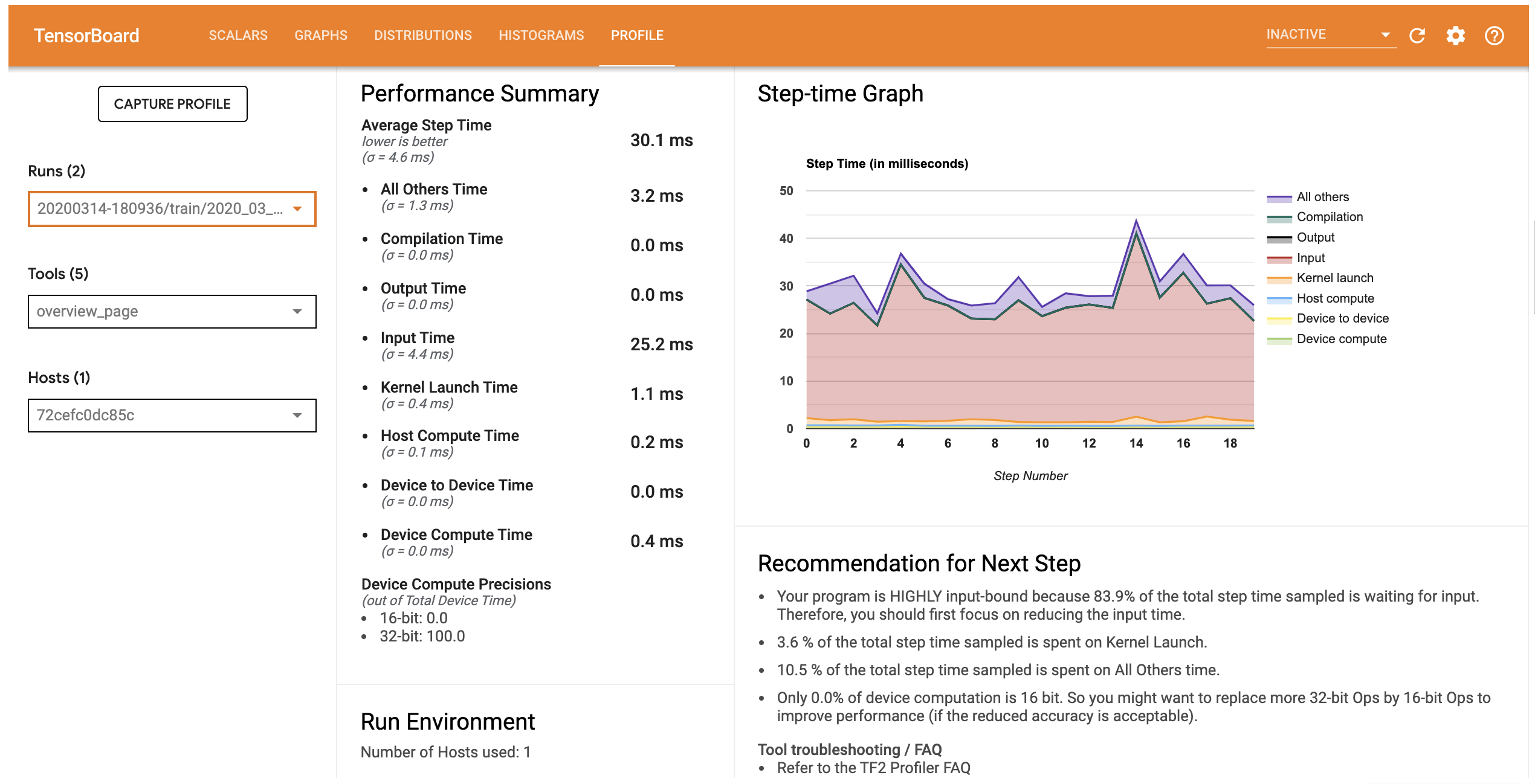
| TensorFlow TensorBoard | ✓ | ✓ | ✓ | ✓ | ✓ | ✗ | ✓ | ✓ | . | ✓ | . |
with:
- ✓ : functionality available and positive impression
- ✗ : functionality available and negative impression (difficult, or current version limited)
- . : functionality absent