

Table des matières
Using Automatic Mixed Precision (AMP) to optimise memory and accelerate calculations
Operational principle
The term «precision» refers here to the way of storing the real variables in memory. Most of the time, the reals are stored on 32 bits. We call them 32-bit floating point reals or Float32, or simple precision. The reals can also be stored on 64 or 16 bits, depending on the desired number of significant digits. We call these Float64 or double precision, and Float16 or semi-precision. The TensorFlow and PyTorch frameworks use simple precision by default but it is possible to exploit the semi-precision format to optimise the learning step.
We speak of mixed precision when we use more than one type of precision in the same model during the forward and backward propagation steps. In other words, we reduce the precision of certain variables of the model during certain steps of the training.
It has been empirically demonstrated that, even in reducing the precision of certain variables, the model learning obtained is equivalent in performance (loss, accuracy) as long as the «sensitive» variables retain the float32 precision by default; this is the same for all the main types of models in current use. In the TensorFlow and PyTorch frameworks, the «sensitivity» of variables is automatically determined by the Automatic Mixed Precision (AMP) functionality. Mixed precision is an optimisation technique for learning. At the end of the optimisation, the trained model is reconverted into float32, its initial precision.
On Jean Zay, you can use AMP while using the Tensor Cores of the NVIDIA V100 GPUs. By using AMP, the computing operations are effectuated more effectively while at the same time keeping an equivalent model.
Comment: Jean Zay also has NVIDIA A100 GPUs on which the Tensor cores can use FP16 and also TF32 (tensor float, equivalent to float32); in this case, you can choose whether or not to use a higher or mixed precision while still using the Tensor cores. Of course, using a lower precision still allows gaining a little more in speed.
Advantages and disadvantages of mixed precision
The following are some advantages of using mixed precision:
- Regarding the memory:
- The model occupies less memory space because we are dividing the size of certain variables in half. 1)
- The bandwidth is less sollicited because the variables are transfered more rapidly into memory.
- Regarding the calculations:
- The operations are greatly accelerated (on the order of 2x or 3x) because of using Tensor cores. The learning time is decreased.
Among classic usage examples, mixed precision is used to:
- Reduce the memory size of a model (which would otherwise exceed the GPU memory size)
- Reduce the learning time of a model (as for large-sized convolutional networks)
- Double the batch size
- Increase the number of epochs
There are few drawbacks to using AMP. There is a very slight lowering of the precision of the trained model (which is fully offset by the gains in memory and calculation) and there is the addition of a few code lines.
AMP effectiveness on Jean Zay
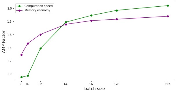
The following figures illustrate the gains in memory and computation times by using mixed precision. These results were measured on Jean Zay for the training of a Resnet50 model on CIFAR and executed in mono-GPU. (1st benchmark with Resnet101)
PyTorch mono-GPU V100 :
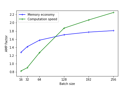
PyTorch mono-GPU A100 :
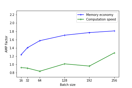
Tensorflow mono-GPU V100 :
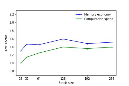
Tensorflow mono-GPU A100 :
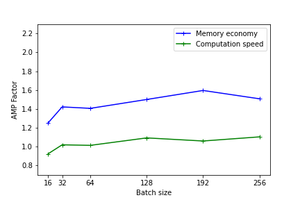
The heavier the model (in terms of memory and operations), the more the usage of mixed precision will be effective. Nevertheless, even for light models, there is an observable performance gain.
On the lightest models, using AMP has no benefit. In fact, the conversion time of the variables can be greater than the gain realized with using Tensor Cores.
The performance is better when the model dimensions (batch size, image size, embedded layers, dense layers) are multiples of 8 due to the specific hardware of Tensor cores as documented on the Nvidia site .
Comment: These tests give an idea of the effectiveness of AMP. The results can be different with other types and sizes of models. Implementing AMP remains the only means of knowing the real gain of your precise model.
In PyTorch
Starting with version 1.6, PyTorch includes the AMP functions (refer to examples on the Pytorch page).
To set up mixed precision and Loss Scaling, it is necessary to add the following lines:
from torch.cuda.amp import autocast, GradScaler

scaler = GradScaler()

for epoch in epochs:
    for input, target in data:
        optimizer.zero_grad()

        with autocast():
            output = model(input)
            loss = loss_fn(output, target)

        scaler.scale(loss).backward()
        scaler.step(optimizer)
        scaler.update()
Important: Before version 1.11: In the case of a distributed code in mono-process, it is necessary to specify the usage of the autocast before defining the forwarding step (see this correction on the Pytorch page). Rather than adding the autocast, we would prefer using one process per GPU as is recommended by distributeddataparallel.
Comment: NVIDIA Apex also offers AMP but this solution is now obsolete and not recommended.
In TensorFlow
Starting with version 2.4, TensorFlow includes a library dedicated to mixed precision:
from tensorflow.keras import mixed_precision
This library enables instantiating mixed precision in the TensorFlow backend. The command line instruction is the following:
mixed_precision.set_global_policy('mixed_float16')
Important: If you use «tf.distribute.MultiWorkerMirroredStrategy», the «mixed_precision.set_global_policy('mixed_float16')» instruction line must be positioned within the context of «with strategy.scope()».
In this way, we indicate to TensorFlow to decide which precision to use at the creation of each variable, according to the policy implemented in the library. The Loss Scaling is automatic when using keras.
If you use a customised learning loop with a GradientTape, it is necessary to explicitly apply the Loss Scaling after creating the optimiser and the Scaled Loss steps (refer to the page of the TensorFlow guide).
Loss Scaling
It is important to understand the effect of converting certain model variables into float16 and to remember to implement the Loss Scaling technique when using mixed precision.
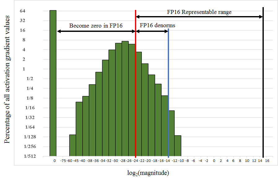
In fact, the representable range of values in float16 precision covers the interval [2-24,215]. However, as we see in the adjacent figure, in certain models the gradient values are well below the lower boundary at the moment of the weight update. They are thus found outside of the representable zone in float16 precision and are reduced to a null value. If we don't do something, the calculations risk being incorrect and a large part of the representable range of values in float16 remains unused.
To avoid this problem, we use a technique called Loss Scaling. During the learning iterations, we multiply the training loss by an S factor to shift the variables towards higher values, representable in Float16. These must then be corrected before updating the model weight by dividing the weight gradients by the same S factor. In this way, we will recover the true gradient values. There are solutions in theTensorFlow and PyTorch frameworks to simplify the process of putting Loss Scaling in place.
1)
There is generally less memory occupation but not in each case. In fact, certain variables are saved both in float16 and float32; this additional data is not necessarily offset by the reduction of other variables in float16.